Voting Simulation Visualizations

This article and all included images are licensed under a Creative Commons Attribution 4.0 International License.

Ka-Ping Yee
posted 2005-04-21, updated 2006-12-08

Among both academics and activists, there has been a long debate over election methods — the rules for marking and counting ballots to determine a winner. The Plurality method, where each voter votes for just one candidate, is the most well known, but it has some problems. Many other possibilities have been proposed; some allow votes for more than one candidate, some ask voters to assign scores or ranks to the candidates, and so on. For a good introduction to election methods, see Wikipedia.

In discussions comparing election methods, people often argue for one method or another by presenting examples of cases where a particular method fails or behaves strangely. There are five commonly cited criteria (called universality, non-imposition, non-dictatorship, monotonicity, and independence of irrelevant alternatives) for "reasonable behaviour" of an election method. But it has been mathematically proven that no single-winner election method can meet all five of these criteria, so one can always invent situations where a particular method violates one of these criteria. Thus, presenting individual cases of strange behaviour proves little.

A more substantive way to argue for or against a particular election method would be to compare how frequently failures occur, under what conditions they occur, and how severe they are. We need a way to map out how an election method behaves over a wide range of cases and understand the effects of a shift in public opinion. I've generated the images on this page in the hope of illustrating these effects better and gaining some insight into how election methods behave.

Simulation Method

The following images were created by simulating a series of single-winner elections under the following assumptions:

• Political opinion is represented by a point on a plane. That is, each voter's position and candidate's position is described by two independent co-ordinates, and the Euclidean distance between two points measures the degree to which two positions differ.
• The voter's positions are distributed according to a bell curve along both dimensions (a two-dimensional Gaussian distribution). The "center of opinion" mentioned below is the center of this distribution.

For each image, the positions of the candidates are fixed. There are three or four candidates, indicated by small circles filled in with the candidate's colour.

Each point in the image corresponds to an election with the center of opinion located at that point. For every point, we simulate an entire election by scattering 200000 voters in a normal distribution around that point and collecting ballots from all of the voters; then we colour the point to indicate the winner.

We present the images five at a time, comparing these election methods:

• Plurality (also called "first past the post"): Each voter may vote for only one candidate. The candidate with the most votes wins.
• Approval: Each voter may vote for any number of candidates. The candidate with the most votes wins.
• Borda: Each voter ranks the candidates in preference order. Candidates get points according to the ranks they are given, and the candidate with the lowest total rank wins.
• Condorcet: Each voter ranks the candidates in preference order. If there is a candidate who would defeat all of the other candidates in one-on-one contests, that candidate wins.
• Hare (also called "instant runoff", "IRV", or "RCV"): Each voter ranks the candidates in preference order. Each ballot is assigned to its highest-ranked candidate, and if one candidate has more than half the ballots, that candidate wins. Otherwise, the candidate with the least first-ranked votes is eliminated, and the ballots ranking that candidate highest are reassigned to the next-highest non-eliminated candidate. The counting and elimination process is repeated until there is a majority winner.

The voters are assumed to vote as follows:

• Plurality: Vote for the nearest candidate.
• Approval: Vote for all the candidates within an acceptable distance. The voters' acceptable distances are randomized according to a log-normal distribution.
• Borda: Rank the candidates in order of increasing distance.
• Condorcet: Rank the candidates in order of increasing distance.
• Hare: Rank the candidates in order of increasing distance.

These are all very simplistic assumptions. They probably do not model real-world voters accurately. However, observing voting methods under these assumptions can show us something about how these voting methods behave. Under these simple assumptions one would expect any reasonable voting method to yield straightforward behaviour; real-world behaviour would only be more complex than what these simulations show.

The following images visually demonstrate how Plurality penalizes centrist candidates and Borda favours them; how Approval and Condorcet yield nearly identical results; and how the Hare method yields extremely strange behaviour. Alarmingly, the Hare method (also known as "IRV" or "RCV") is gaining momentum as the most popular type of election-method reform in the United States (in Berkeley, Oakland, and just last November in San Francisco, for example).

Three Candidates

In each group of five images, the three candidates (red, green, and blue) all have the same positions. In all the images, the x-axis ranges from -0.25 to 1.25 (left to right) and the y-axis ranges from -0.25 to 1.25 (bottom to top). The Gaussian distribution of voters has a sigma of 0.5.

Equilateral

The three candidates are positioned in an equilateral triangle: red at (0.5, 0.99), green at (0.07, 0.25), and blue at (0.93, 0.25). As one might expect, all voting systems treat them fairly. That is, when the center of opinion is nearest the red candidate, the red candidate wins; when it is nearest the blue candidate, the blue candidate wins; when it is nearest the green candidate, the green candidate wins.

Squeezed Out

In this example, we have red at (0.07, 0.17), green at (0.49, 0.01), and blue at (0.41, 0.02). Here we start to see some problems. The Plurality and Hare (IRV) methods both favour extremists: they can squeeze out a moderate candidate. The blue candidate, stuck in the middle between the red and green candidates, will win when public opinion is moderate with the Approval and Condorcet methods, but has no chance of winning in the Plurality and Hare methods. The blue candidate has an even larger winning region with the Borda method.

Vote Splitting

Here is a visual illustration of splitting the vote. Red is located at (0.93, 0.49), green at (0.79, 0.42), and blue at (0.27, 0.45). If the red candidate were not running, then the contest between blue and green should split exactly halfway between the two candidates, as it does in Approval and Condorcet. Notice that in Plurality voting, the addition of the red candidate has caused the blue region to expand to the right: blue has gained an unfair advantage because red and green are splitting the vote. This is a commonly cited problem with Plurality voting, and a strong motivator for voting reform. With Borda voting, the result is the opposite: the presence of the red candidate is actually helpful to the green candidate, expanding the green winning region slightly.

Nonmonotonicity

In the previous example, the plot for IRV shows a concave, M-shaped green region. When a candidate's winning region is concave, that means the election method is nonmonotonic. That is, a shift of public opinion toward a candidate can cause the candidate to lose, and a shift of public opinion away from a candidate can cause the candidate to win. Here is a more extreme example of such pathological behaviour. Red is located at (0.54, 0.47), green at (0.77, 0.64), and blue at (0.13, 0.10). Look at the image in the lower-left for IRV, which shows a red region with two spikes. When the center of opinion is located in the left spike, moving toward the red candidate can cause red to lose. When the center of opinion is located in the right spike, moving away from the green candidate can cause green to win.

Four Candidates

In each group of five images, the four candidates (red, green, yellow, and blue) all have the same positions. In all the images, the x-axis ranges from -0.25 to 1.25 (left to right) and the y-axis ranges from -0.25 to 1.25 (bottom to top). The Gaussian distribution of voters has a sigma of 0.5.

Square

For four candidates in a perfect square (red, yellow, green, and blue at (0.3, 0.3), (0.7, 0.3), (0.3, 0.7), and (0.7, 0.7) respectively), Plurality, Approval, Borda, and Condorcet yield the obvious expected outcomes here. But even in this simplest of cases, IRV behaves unreasonably. The strange colours in the center of the figure are caused by counting the second-place choices of only some voters and disregarding others. For example, the red and blue areas in the upper-left quadrant are due to large numbers of voters who rank yellow highest; when yellow is eliminated first, their ballots count as votes for red or blue.

Shattered

Here we have red at (0.12, 0.28), yellow at (0.85, 0.70), green at (0.39, 0.28), and blue at (0.97, 0.14). Plurality severely penalizes green, the moderate. The Approval and Condorcet methods yield boundaries exactly halfway between candidates, and once again, the centrist gets the largest winning region with Borda. The IRV method yields a very strange shape for green's winning region.

Disjoint

In this example, red is located at (0.24, 0.23), yellow at (0.19, 0.62), green at (0.04, 0.64), and blue at (0.85, 0.55). Again, Plurality works against the moderate and Borda favours the moderate. The IRV method divides the yellow candidate's winning area into two disjoint regions.

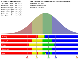
Nonmonotonicity City

This example demonstrates more absurd behaviour from the IRV method. Red is at (0.40, 0.57), yellow at (0.16, 0.54), green at (0.05, 0.62), and blue at (0.91, 0.70).